Ehtereum Network Analysis — Part 04: Network Construction

In this part, I finally start building the actual Ethereum transaction networks based on the cleaned data from Part 02 and the basic statistics from Part 03. Even though I only selected one day of data (2025‑11‑11), the dataset is still large enough to construct meaningful ETH graphs, token graphs, and heterogeneous multi-graphs. The idea here is not to chase long-term patterns, but to build a reproducible pipeline.

1. ETH Transfer Graph

As usual, Ethereum is naturally a graph.
Nodes = addresses.
Edges = ETH transfers.

1.1 Load Data

df_eth = pd.read_csv("data/cleaned/eth_transfers_cleaned.csv")
df_eth.head()

1.2 Build Graph

import networkx as nx

G_eth = nx.DiGraph()

for _, row in df_eth.iterrows():
    G_eth.add_edge(
        row["from"],
        row["to"],
        value=row["value"],
        timestamp=row["timeStamp"],
        tx_hash=row["hash"]
    )

1.3 ETH Graph Statistics

At first glance, the ETH transfer graph is relatively small compared to token transfers, which is expected since many activities happen via tokens. We can see from the talbe below some basic statistics. | Metric | Value | |—————|——–| | Nodes | ~7.8k | | Edges | ~9.2k | | Avg Degree | 2.37 | | Max Degree | 417 |

Interms of conntected components, the ETH graph is mostly connected, with a giant component covering most nodes. Below are some stats: | Metric | Value | |————————-|——–| | Weakly Connected Comps | 557 | | Strongly Connected Comps | 6748 | | Largest WCC Size | 6315 |
Usually, usually, the lagest WCC proportion is more than 95% in Ethereum networks.

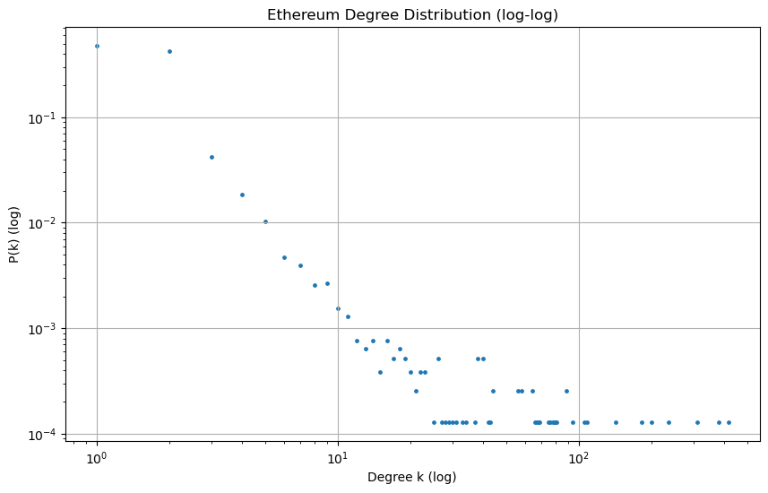
Degree distribution also shows a long tail, with a few addresses having very high degrees (mostly exchanges and popular contracts). Log-log plot below:

1.4 ETH Graph Sample Visualization

I cannot plot the full graph (obviously), so I use subgraphs. Here is a High-Degree Ego Graph Sample with top 300 nodes by degree:

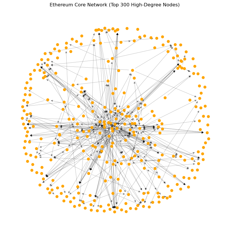
We can see some well-known exchange addresses and smart contract addresses in the center of the graph, acting as hubs for ETH transfers.

---

2. Token Transfer Graph

Token transfers behave differently from ETH transfers.
This is where most activity happens.

2.1 Build Token Graph

G_token = nx.DiGraph()

for _, row in df_token.iterrows():
    G_token.add_edge(
        row["from"],
        row["to"],
        token=row["tokenSymbol"],
        value=row["value"],
        timestamp=row["timeStamp"]
    )

2.2 Token Statistics

User transfers predominate, with only a few token contracts (USDC, USDT, WETH) involved. | Metric | Value | |—————|——–| | Nodes | ~24.6k | | Edges | ~21.4k | | Avg Degree | 1.73 | | Token Contracts | 3 | —

3. Heterogeneous Multi-Graph

Now I merge ETH and tokens into one heterogeneous network.

3.1 Build MultiDiGraph

G = nx.MultiDiGraph()

Number of contract addresses: 2826 Number of EOA addresses: 7440 Total number of nodes in the graph: 10266

3.2 Random Subgraph Visualization

From the visualization, a circle shape indicates a contract address, while a square shape indicates an EOA address. The colors represent different types of transfers: blue for ETH transfers and orange for token transfers. The size of the nodes corresponds to their degree, highlighting the more connected addresses in the network.

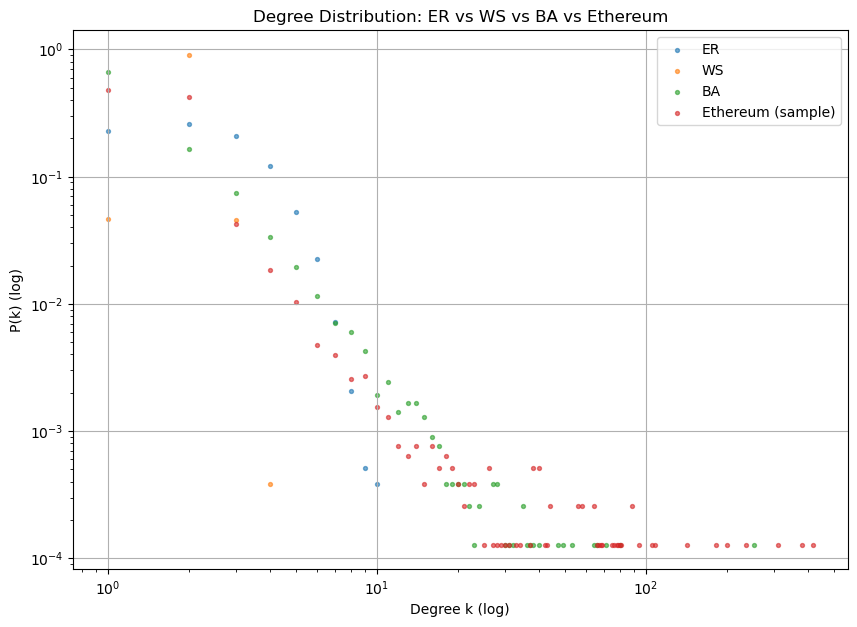
4. Theoretical vs. Actual Edge Counts

ER vs WS vs BA vs Ethereum To understand the structure of the Ethereum network better, I compared the actual edge counts with theoretical models like Erdős-Rényi (ER), Watts-Strogatz (WS), and Barabási-Albert (BA) models.

It is not very

5. Summary

Even one day of Ethereum activity is enough to build large-scale networks.
The pipeline is solid, and the next step is to analyze global structure.

Stay tuned for next part!