
Market Fear Regime Identification - Part1: Introduction
Project Overview
Motivation
Interactive Demo: Check out the live visualization to explore the market regimes and event analysis.
The cryptocurrency market is known for extreme volatility and sentiment-driven price movements. Unlike traditional financial markets with decades of regulatory oversight, crypto markets shift between regimes quickly — from extreme fear (panic selling, high correlations) to extreme greed (FOMO rallies, overconfidence).
The core challenge is identifying these market regimes without labeled historical data. Traditional supervised learning needs annotated examples (“this period was fear”, “that period was greed”), but such labels are subjective and don’t exist at scale. This project uses an unsupervised learning approach, applying clustering algorithms to discover latent market states from quantitative features.
Objectives
This project tries to identify market regimes (fear, neutral, greed, and so on) using K-Means clustering. I’m combining quantitative features like volatility and returns with sentiment data from the Fear & Greed Index. The goal is to validate this approach with a minimal feature set before scaling to multi-asset analysis, visualize how regimes evolve over time, and build a foundation for more advanced network analysis later.
Why This Matters
Detecting fear regimes early helps with risk management — you can reduce exposure before crashes. Regime-aware trading strategies can adapt to market conditions (like trend-following during greed phases, mean-reversion during fear). This also demonstrates how unsupervised learning works in financial time series without arbitrary labels, and sets up analysis of how asset correlations change across regimes.
Technical Stack
I’m using Yahoo Finance (yfinance) and the Alternative.me API for the Fear & Greed Index. Probably expend to other data sources later. The core libraries are pandas, numpy, and scikit-learn (K-Means, StandardScaler, evaluation metrics). Visualization is done with matplotlib. Working environment is Jupyter Notebook with Python 3.11+ in a conda environment.
Data Pipeline
Asset Selection
I started with 20 cryptocurrencies selected from CoinGecko’s top market cap rankings. The core assets include BTC, ETH, BNB, SOL, XRP, ADA, DOGE, DOT, LTC, and TRX. Supplementary assets are AVAX, MATIC, LINK, ATOM, UNI, ETC, XLM, ALGO, FIL, and APT.
The rationale is straightforward: BTC serves as the market benchmark (highest correlation with overall sentiment), and I wanted a mix of Layer-1 blockchains (ETH, SOL, ADA), DeFi tokens (UNI, LINK), and even meme coins (DOGE). This gives enough diversity for future network analysis while keeping the data manageable.
Data Fetching
The data comes from Yahoo Finance via the yfinance library, covering 2018-01-01 to present — over 7 years spanning multiple bull and bear cycles. I’m using daily OHLCV (Open, High, Low, Close, Volume) data.
#
import yfinance as yf

tickers = ['BTC-USD', 'ETH-USD', 'BNB-USD', ...]  # yfinance requires '-USD' suffix
data = yf.download(tickers, start='2018-01-01', end='2024-11-27',
                   group_by='ticker', auto_adjust=True)
A few challenges came up. First, yfinance returns MultiIndex DataFrames with nested columns (ticker, price_type), which requires careful extraction. Some altcoins lack early historical data — SOL only launched in 2020, for example. I also had to ensure the Fear & Greed Index timestamps align with price data to avoid look-ahead bias.
Sentiment Data Integration
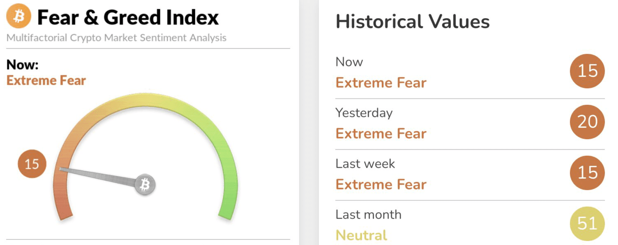
The sentiment data comes from the Alternative.me Crypto Fear & Greed Index API (https://api.alternative.me/fng/?limit=0&date_format=world). This index aggregates several signals: volatility (25% weight), market momentum and volume (25%), social media sentiment (15%), surveys (15%), Bitcoin dominance as a risk-off indicator (10%), and Google Trends search volume (10%). The index ranges from 0 (Extreme Fear) to 100 (Extreme Greed).
import requests
import pandas as pd

response = requests.get('https://api.alternative.me/fng/?limit=0&date_format=world')
fg_data = pd.DataFrame(response.json()['data'])
fg_data['date'] = pd.to_datetime(fg_data['timestamp'], unit='s')
fg_data['fg_raw'] = fg_data['value'].astype(int)
Data Cleaning & Alignment
I merged the price matrix and Fear & Greed data on the date column. For missing values, I forward-filled minor gaps (less than 3 days) and dropped rows for extended missing periods to preserve data quality. The Fear & Greed Index gets scaled to [0, 1] by dividing by 100. Price features will be standardized later after feature engineering.
The output files are data/row/price_matrix.csv (raw OHLCV data for all tickers) and data/processed/full_market_matrix.csv (aligned price plus Fear & Greed data, ready for feature engineering).
For data quality, I checked that there are no duplicate dates, the date index is monotonic, Fear & Greed coverage spans 2018-01-01 to present with 100% overlap with price data, and BTC as the anchor has complete data across the full time range.
Sample of Processed Data
| ADA | ALGO | APT | ATOM | AVAX | BNB | BTC | DOGE | DOT | ETC | ... | MATIC | SOL | TRX | UNI | XLM | XRP | fg_raw | ret_btc | vol_btc_7 | fg_norm | |
|---|---|---|---|---|---|---|---|---|---|---|---|---|---|---|---|---|---|---|---|---|---|
| date | |||||||||||||||||||||
| 2025-11-22 | 0.404608 | 0.135694 | 0.000131 | 2.509819 | 13.227550 | 833.351074 | 84648.359375 | 0.140304 | 2.309507 | 13.499508 | ... | 0.216415 | 127.551201 | 0.274130 | 0.000163 | 0.230294 | 1.949751 | 11.0 | -0.005212 | 0.370388 | 0.11 |
| 2025-11-23 | 0.408549 | 0.143644 | 0.000131 | 2.492277 | 13.277553 | 843.224792 | 86805.007812 | 0.144831 | 2.255722 | 13.556331 | ... | 0.216415 | 130.705063 | 0.275073 | 0.000163 | 0.247030 | 2.046265 | 13.0 | 0.025159 | 0.482436 | 0.13 |
| 2025-11-24 | 0.427842 | 0.143671 | 0.000131 | 2.501120 | 13.890861 | 864.421143 | 88270.562500 | 0.151794 | 2.339354 | 14.159579 | ... | 0.216415 | 138.371353 | 0.274809 | 0.000163 | 0.254841 | 2.225878 | 19.0 | 0.016742 | 0.511347 | 0.19 |
| 2025-11-25 | 0.421617 | 0.146376 | 0.000131 | 2.465958 | 14.169900 | 862.108032 | 87341.890625 | 0.152972 | 2.294471 | 14.156011 | ... | 0.216415 | 138.891144 | 0.274355 | 0.000163 | 0.251900 | 2.198544 | 20.0 | -0.010576 | 0.495043 | 0.20 |
| 2025-11-26 | 0.435622 | 0.146284 | 0.000131 | 2.526135 | 14.936302 | 891.753357 | 90518.367188 | 0.154778 | 2.344442 | 14.134871 | ... | 0.216415 | 143.012192 | 0.276516 | 0.000163 | 0.258838 | 2.224285 | 15.0 | 0.035723 | 0.582807 | 0.15 |
5 rows × 24 columns
Next Steps
The next post will cover feature engineering: calculating daily log returns, rolling volatility, and normalizing the Fear & Greed Index. After that, I’ll implement K-Means clustering to identify market regimes and visualize how these regimes evolve over time.