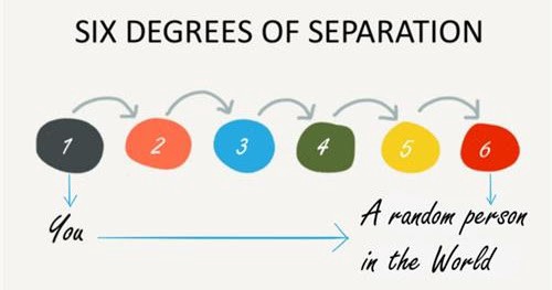
Six Degrees of Separation - Initial Exploration

Curiosity · Craft · Simplicity — “Build to wonder.”

Today I heard my teacher casually mention this idea: how many people would it take, at minimum, to reach a specific stranger?
My mind jumped to that old rule of thumb — was it five people, or six?
I’ve known about it for years, but I never asked why it might be true.
So, here we are. Let’s explore.

I wanted this piece to explore a little bit. I’ll build a tiny “social world” in Python, see how short paths emerge, and then peek under the hood with a friendly bit of linear algebra. Nothing heavy; just enough to see the shape of the idea.

---

Why six, anyway? (the intuition)

If you squint at society, it looks like a web: clusters of friends connected by a few long bridges. Most of your friends know each other — that’s the clustering part. But a handful of “weak ties” reach far — those are the bridges. Put both together and you get a small world: most people are only a few handshakes apart.

That’s the intuition. Now let’s build a toy world and see it.

WIKIPEDIA-SixDegrees

What we’ll build

1) A small-world network (using the classic Watts–Strogatz model).
2) Pick two random people and highlight the shortest path between them.
3) Convert the graph to an adjacency matrix $A$, and use powers of $A$ to read “how many steps away” relationships are.
4) Measure a few friendly metrics: average path length, diameter, clustering coefficient.

---

Setup (one minute)

pip install networkx matplotlib numpy

Any Python 3 environment will do. If you’re using Jupyter or VS Code, run each section in its own cell so you can glance at the output comfortably.

---

Part I — Draw a tiny world and walk a path

We’ll start with the Watts–Strogatz model: it begins as a tidy ring (everyone knows a few close neighbors), then randomly rewires some edges (creating those long bridges). That mix typically yields short paths and high clustering — a nice cartoon of real-life networks.

import networkx as nx
import matplotlib.pyplot as plt
import random

# 1) Build a small-world social graph
n, k, p = 30, 4, 0.3  # 30 people; each knows ~4 neighbors; 30% chance to rewire = some long ties
G = nx.watts_strogatz_graph(n=n, k=k, p=p, seed=42)

# 2) Pick two people at random
a, b = random.sample(G.nodes(), 2)

# 3) Shortest path (our "degrees of separation")
path = nx.shortest_path(G, source=a, target=b)
degree = len(path) - 1

print(f"Person  → Person ")
print("Path:", path)
print("Degrees of separation:", degree)

# 4) Visualize
plt.figure(figsize=(8, 6))
pos = nx.spring_layout(G, seed=42)  # neat, consistent layout
nx.draw_networkx_nodes(G, pos, node_size=400, node_color="lightblue", alpha=0.9)
nx.draw_networkx_edges(G, pos, width=1.2, alpha=0.6)
nx.draw_networkx_labels(G, pos, font_size=9)

# Highlight the shortest path
nx.draw_networkx_nodes(G, pos, nodelist=path, node_size=600, node_color="tomato")
nx.draw_networkx_edges(G, pos, edgelist=list(zip(path, path[1:])), edge_color="red", width=2.5)

plt.title(f"Six Degrees Demo (n=, k=, p=)\n → , degrees = ")
plt.axis("off")
plt.tight_layout()
plt.show()

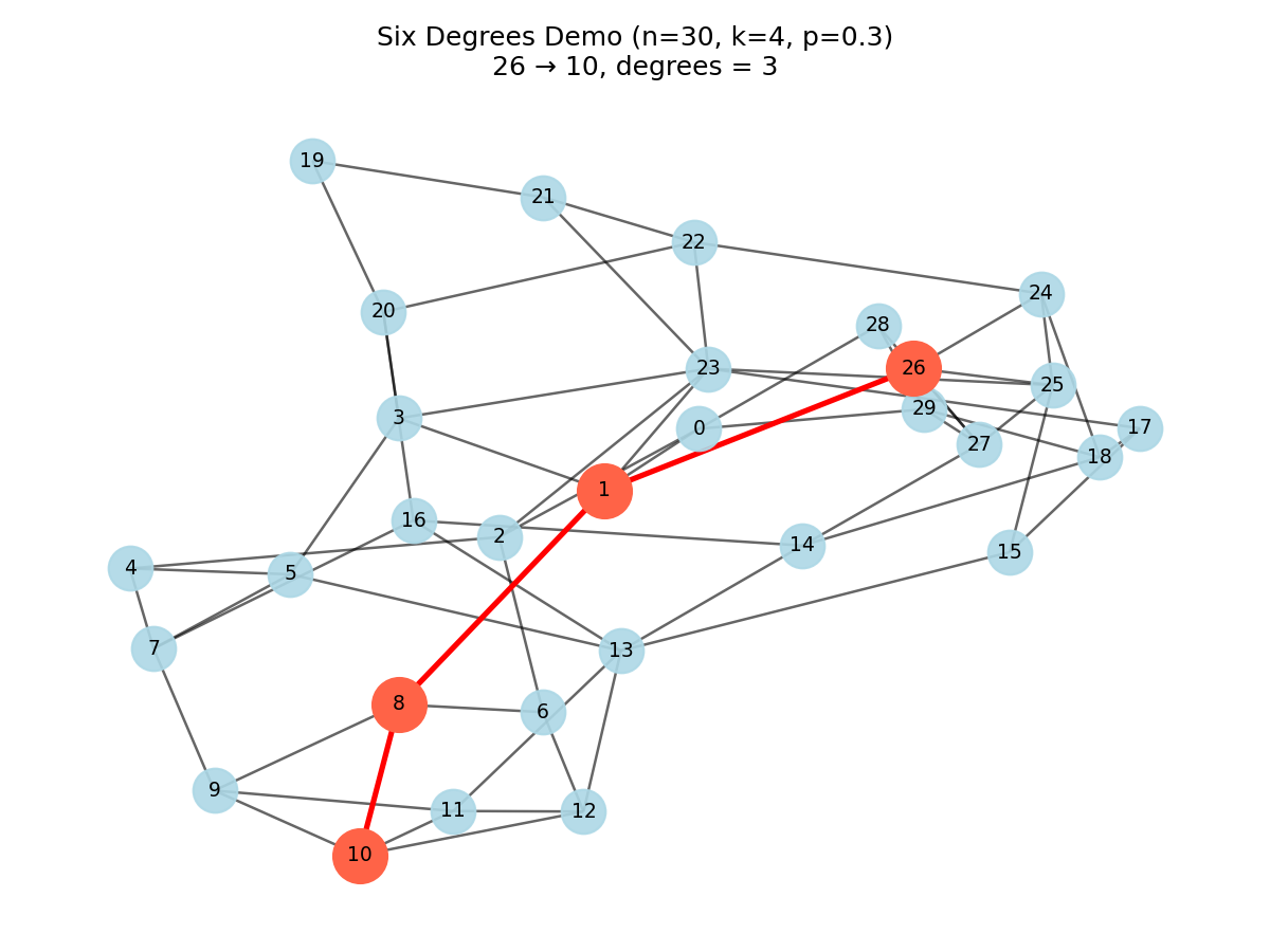
— Caption: The red route is the “few handshakes away” path.

A few notes, human to human:

• If k is too small, the graph can break into islands (not everyone is reachable).
• If k is huge, everyone knows everyone — not very interesting.
• A modest rewiring p (say, 0.1–0.3) introduces just enough long ties to shrink distances dramatically.

---

Part II - A friendly peek at the matrix

Let’s turn the picture into a matrix.
The adjacency matrix $A$ is a table where $A_{ij} = 1$ if person $i$ knows person $j$, else $0$.
Here’s the quiet magic:

• $A^2_{ij}$: number of ways to reach $j$ from $i$ in exactly 2 steps.
• $A^3_{ij}$: same for 3 steps.
• More generally, $A^k$ encodes “paths of length $k$”.

So if any of $A, A^2, \dots, A^6$ has a positive entry at $(i, j)$, then $i$ can reach $j$ within six steps — and that’s the heart of the “six degrees” idea.

import numpy as np

# Adjacency matrix as 0/1 integers (easier on the eyes)
A = nx.to_numpy_array(G, dtype=int)
print("Adjacency matrix A:\n", A)

# Powers of A — read as "paths of length k"
powers = {}
for k_step in range(2, 7):
    Ak = np.linalg.matrix_power(A, k_step)
    powers[k_step] = Ak
    print(f"\nA^{k_step} (exact {k_step}-step paths):\n", Ak)

# Within six steps? Sum A^1..A^6 and check > 0
A_sum_1_to_6 = sum(np.linalg.matrix_power(A, i) for i in range(1, 7))
reachable_1_to_6 = (A_sum_1_to_6 > 0).astype(int)

n = A.shape[0]
offdiag = ~np.eye(n, dtype=bool)
ratio = reachable_1_to_6[offdiag].mean()
print(f"Within six steps, reachable pair ratio: {ratio:.2%}")

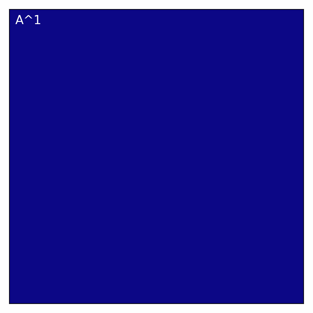
— Caption: As k grows, more off-diagonal entries turn “on”. The world shrinks.

This is all the linear algebra we need.

---

Part III — Numbers for your gut: small-world metrics

A network “feels small” when most pairs are close, and local friendship triangles are common.

# Compute metrics on the largest connected component (safer if G is fragmented)
if not nx.is_connected(G):
    largest_cc_nodes = max(nx.connected_components(G), key=len)
    H = G.subgraph(largest_cc_nodes).copy()
else:
    H = G

avg_path_len = nx.average_shortest_path_length(H)
diameter = nx.diameter(H)
clustering = nx.average_clustering(H)

print("[Small-world metrics on the largest component]")
print(f"Average shortest path length: {avg_path_len:.3f}")
print(f"Diameter (max shortest path): {diameter}")
print(f"Average clustering coefficient: {clustering:.3f}")

Within six steps, reachable pair ratio: 
[Small-world metrics on the largest component]
Average shortest path length: 2.607
Diameter (max shortest path): 5
Average clustering coefficient: 0.197

— Caption: Short paths + high clustering = small world vibes.

degree distribution — who are the social hubs?

degrees = [deg for _, deg in G.degree()]
plt.figure(figsize=(6,4))
plt.hist(degrees, bins=range(min(degrees), max(degrees)+2), alpha=0.85, rwidth=0.9)
plt.xlabel("Degree (how many people someone knows)")
plt.ylabel("Count")
plt.title("Degree distribution")
plt.tight_layout()
plt.show()

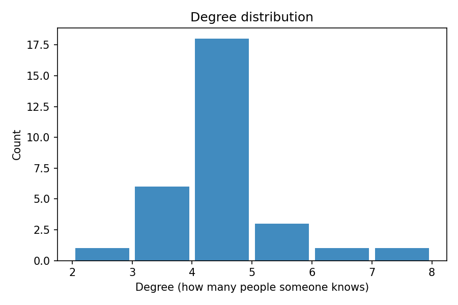
— Caption: A few well-connected people quietly bridge the crowd.

---

Part IV — Tweak, feel, repeat

We can try different parameters and see how the small-world vibe changes.

• Turn the knob: sweep p from 0 → 0.5. Watch average path length collapse while clustering stays pleasantly high for a while.
• Scale up: bump n to 100 or 300. The story persists: short paths survive.

Anyway, I’m tired writing more here. It’s time to enjony the scene of Dolomites at sunset.

Have fun exploring!

---

A quiet wrap-up

If you try this with real data — email graphs, coauthor networks, or even your own friend circles — the numbers will move, but the feeling tends to stay.

---

Appendix — complete script

Tell me you have some interest insights

import networkx as nx
import matplotlib.pyplot as plt
import random

# 1) Build a small-world social graph
n, k, p = 30, 4, 0.3  # 30 people; each knows ~4 neighbors; 30% chance to rewire = some long ties
n, k, p = 300, 4, 0.5  # 30 people; each knows ~4 neighbors; 30% chance to rewire = some long ties
G = nx.watts_strogatz_graph(n=n, k=k, p=p, seed=42)

# 2) Pick two people at random
a, b = random.sample(G.nodes(), 2)

# 3) Shortest path (our "degrees of separation")
path = nx.shortest_path(G, source=a, target=b)
degree = len(path) - 1

print(f"Person to Person ")
print("Path:", path)
print("Degrees of separation:", degree)

# 4) Visualize
plt.figure(figsize=(8, 6))
pos = nx.spring_layout(G, seed=42)  # neat, consistent layout
nx.draw_networkx_nodes(G, pos, node_size=400, node_color="lightblue", alpha=0.9)
nx.draw_networkx_edges(G, pos, width=1.2, alpha=0.6)
nx.draw_networkx_labels(G, pos, font_size=9)

# Highlight the shortest path
nx.draw_networkx_nodes(G, pos, nodelist=path, node_size=600, node_color="tomato")
nx.draw_networkx_edges(G, pos, edgelist=list(zip(path, path[1:])), edge_color="red", width=2.5)

# plt.title(f"Six Degrees Demo (n=, k=, p=)\n → , degrees = ")
plt.title(f"Six Degrees Demo (n={n}, k={k}, p={p})\n{a} → {b}, degrees = {degree}")
plt.axis("off")
plt.tight_layout()
plt.savefig("six_degrees_demo.png", dpi=150)
plt.show()


import numpy as np

# Adjacency matrix as 0/1 integers (easier on the eyes)
A = nx.to_numpy_array(G, dtype=int)
print("Adjacency matrix A:\n", A)

# Powers of A — read as "paths of length k"
powers = {}
for k_step in range(2, 7):
    Ak = np.linalg.matrix_power(A, k_step)
    powers[k_step] = Ak
    print(f"\nA^{k_step} (exact {k_step}-step paths):\n", Ak)

# Within six steps? Sum A^1..A^6 and check > 0
A_sum_1_to_6 = sum(np.linalg.matrix_power(A, i) for i in range(1, 7))
reachable_1_to_6 = (A_sum_1_to_6 > 0).astype(int)

n = A.shape[0]
offdiag = ~np.eye(n, dtype=bool)
ratio = reachable_1_to_6[offdiag].mean()
print(f"Within six steps, reachable pair ratio: ")



import matplotlib.pyplot as plt
import matplotlib.animation as animation
import numpy as np
import networkx as nx

# build graph and adjacency matrix
G = nx.watts_strogatz_graph(30, 4, 0.3, seed=42)
A = nx.to_numpy_array(G, dtype=int)

# generate adjacency matrix powers A^1 to A^6
mats = [np.linalg.matrix_power(A, k) for k in range(1, 7)]

# plot setup
fig, ax = plt.subplots(figsize=(5, 5))
im = ax.imshow(mats[0], cmap="plasma", vmin=0, vmax=max(m.max() for m in mats))

txt = ax.text(0.02, 0.95, "A¹", color="white", fontsize=14, transform=ax.transAxes)


ax.set_xticks([])
ax.set_yticks([])


def update(frame):
    mat = mats[frame]
    im.set_array(mat)
    txt.set_text(f"A^{frame+1}")
    return [im, txt]

# create animation
ani = animation.FuncAnimation(
    fig, update, frames=len(mats), interval=1000, blit=True, repeat=True
)

plt.tight_layout()

# 
ani.save("adjacency_powers_animation.gif", writer="pillow", fps=1)

plt.show()



# Compute metrics on the largest connected component (safer if G is fragmented)
if not nx.is_connected(G):
    largest_cc_nodes = max(nx.connected_components(G), key=len)
    H = G.subgraph(largest_cc_nodes).copy()
else:
    H = G

avg_path_len = nx.average_shortest_path_length(H)
diameter = nx.diameter(H)
clustering = nx.average_clustering(H)
print("[Small-world metrics on the largest component]")
print(f"Average shortest path length: {avg_path_len:.3f}")
print(f"Diameter (max shortest path): {diameter}")
print(f"Average clustering coefficient: {clustering:.3f}")


# Degree distribution plot
degrees = [deg for _, deg in G.degree()]
plt.figure(figsize=(6,4))
plt.hist(degrees, bins=range(min(degrees), max(degrees)+2), alpha=0.85, rwidth=0.9)
plt.xlabel("Degree (how many people someone knows)")
plt.ylabel("Count")
plt.title("Degree distribution")
plt.tight_layout()
plt.savefig("degree_distribution.png", dpi=150)
plt.show()