
Trapezoidal Rule with OpenMP: critical vs. reduction
“High performance computing is a perfect tool to accelerate numerical methods, but getting the parallel patterns right can be tricky. In this post, I explore two common OpenMP approaches to parallelizing the trapezoidal rule for numerical integration.”
In this post I’ll walk through how I implemented the trapezoidal rule for numerical integration in C, and then parallelized it using OpenMP in two different ways:
parallel + for + criticalparallel for + reduction
They both compute the same mathematical thing, but the way they use threads — and the performance implications — are quite different.
I’ll try to keep it simple.
1. The problem: approximate a definite integral
The basic numerical analysis problem is:
\[I = \int_a^b f(x)\, dx\]We want a numerical approximation of this integral. To keep the example simple (and testable), I’ll use:
\[f(x) = x^2,\quad a = 0,\quad b = 1\]The nice thing about this choice is that we know the exact answer:
\[\int_0^1 x^2 dx = \left[\frac{x^3}{3}\right]_0^1 = \frac{1}{3} \approx 0.3333333333\ldots\]So later, when we print the result of our program, we can directly see if it looks reasonable or not.
2. Recap: the trapezoidal rule
Let’s briefly recall what the trapezoidal rule is doing.
I always like to picture it geometrically first.
2.1 Slicing the interval
We split the interval $[a, b]$ into $n$ subintervals of equal width:
\[h = \frac{b - a}{n}\]This gives us the grid points:
\[x_0 = a,\quad x_1 = a + h,\quad x_2 = a + 2h,\ \ldots,\ x_n = a + nh = b\]At each $x_i$, we evaluate the function $f(x_i)$.
2.2 A single trapezoid
On each small subinterval $[x_i, x_{i+1}]$, we approximate the curve by a straight line between $(x_i, f(x_i))$ and $(x_{i+1}, f(x_{i+1}))$.
This forms a trapezoid with:
- height (base in the x‑direction): $h$
- two parallel sides (in the y‑direction): $f(x_i)$ and $f(x_{i+1})$
The area of this trapezoid is:
\[\text{Area}_i = \frac{h}{2} \big( f(x_i) + f(x_{i+1}) \big)\]2.3 Summing all trapezoids
Now we just add up all these small trapezoids:
\[I \approx \sum_{i=0}^{n-1} \frac{h}{2}\,\big(f(x_i) + f(x_{i+1})\big)\]If you expand and regroup terms, you get the classic “endpoints once, middle points twice” formula:
\[I \approx \frac{h}{2} \left[ f(x_0) + 2 f(x_1) + 2 f(x_2) + \cdots + 2 f(x_{n-1}) + f(x_n) \right].\]In the form that is most convenient for coding:
\[I \approx h\left( \frac{f(x_0) + f(x_n)}{2} + \sum_{i=1}^{n-1} f(x_i) \right).\]That last line is almost a direct translation into C: compute the two endpoints once, sum all the middle points, and multiply by $h$.
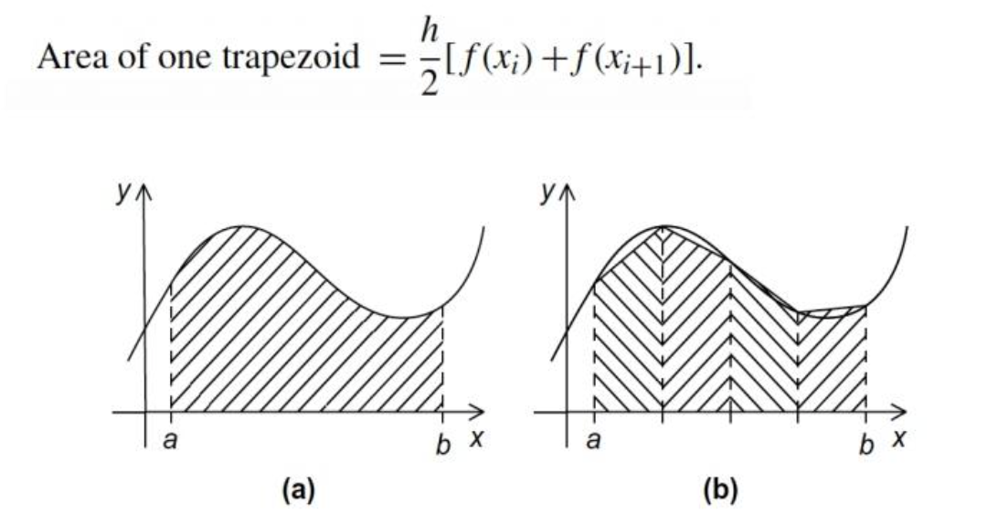
3. Visual intuition: trapezoids under the curve
Here’s a simple diagram to visualize what’s going on.
%% Conceptual illustration of the trapezoidal rule
graph LR
    A[x0] --> B[x1] --> C[x2] --> D[x3] --> E[x4]

    subgraph "f(x) sampled at grid points"
    A1(( )):::point
    B1(( )):::point
    C1(( )):::point
    D1(( )):::point
    E1(( )):::point
    end

    A -. f(x0) .- A1
    B -. f(x1) .- B1
    C -. f(x2) .- C1
    D -. f(x3) .- D1
    E -. f(x4) .- E1

    A1 --- B1 --- C1 --- D1 --- E1

    classDef point fill:#f5d6a0,stroke:#c97f00,stroke-width:2px;
The idea is:
- More slices (larger $n$) → trapezoids become thinner → approximation improves.
- For our OpenMP experiments, we’ll typically pick a large $n$ (like 1,000,000) so that there is enough work to see the benefit of parallelism.
4. Baseline: a serial implementation in C
Before doing anything with OpenMP, I always like to write a clean serial version.
This is both a correctness reference and a performance baseline.
#include <stdio.h>

double f(double x) {
    return x * x;   // Example function: f(x) = x^2
}

int main() {
    double a = 0.0;
    double b = 1.0;
    int n = 1000000;   // number of subintervals

    double h = (b - a) / n;
    double sum = 0.0;

    // Endpoint contribution: (f(a) + f(b)) / 2
    sum += (f(a) + f(b)) / 2.0;

    // Sum over interior points: i = 1 .. n-1
    for (int i = 1; i < n; i++) {
        double x = a + i * h;
        sum += f(x);
    }

    double result = h * sum;

    printf("Integral (serial) = %.15f\n", result);
    return 0;
}
Expected output (roughly):
Integral (serial) = 0.333333333333xxx
If that number is too far from 1/3, something is wrong.
5. First parallel version: parallel + for + critical
Now we start using OpenMP.
The critical part of our serial code is the loop:
for (int i = 1; i < n; i++) {
    double x = a + i * h;
    sum += f(x);
}
The good news: each iteration is independent (no dependence on other i).
The bad news: all iterations update the same variable sum.
So the plan is:
- Let each thread have its own local accumulator
local_sum. - Use
#pragma omp forto split the iterations among threads. - After a thread is done with its iterations, it enters a critical region to safely add
local_sumto the sharedsum.
5.1 Why not just do sum += f(x) in parallel?
Because that would look like this:
#pragma omp parallel for
for (int i = 1; i < n; i++) {
    double x = a + i * h;
    sum += f(x);   // <-- dangerous!
}
Multiple threads would try to update sum at the same time → race condition.
You might see weird results or non‑deterministic behavior.
So we really want to separate:
- independent computation (
local_sum += f(x);) - shared update (
sum += local_sum;) protected withcritical
5.2 Code: trapezoidal rule with parallel + for + critical
Here is the full version using OpenMP in this style:
#include <stdio.h>
#include <omp.h>

double f(double x) {
    return x * x;   // Example: f(x) = x^2
}

int main() {
    double a = 0.0;
    double b = 1.0;
    int n = 1000000;

    double h = (b - a) / n;
    double sum = 0.0;

    // Endpoint contribution: (f(a) + f(b)) / 2
    sum += (f(a) + f(b)) / 2.0;

    // Parallel region
    #pragma omp parallel
    {
        double local_sum = 0.0;  // Each thread has its own local sum

        // Distribute the loop iterations among threads
        #pragma omp for
        for (int i = 1; i < n; i++) {
            double x = a + i * h;
            local_sum += f(x);
        }

        // Safely accumulate into the shared sum
        #pragma omp critical
        {
            sum += local_sum;
        }
    } // end of parallel region

    double result = h * sum;

    printf("Integral (parallel + critical) = %.15f\n", result);
    return 0;
}
If you run this with different thread counts, you should see roughly the same numerical result as the serial version, but potentially less runtime when n is large and your CPU has multiple cores.
For example:
gcc -fopenmp trap_critical.c -o trap_critical

OMP_NUM_THREADS=1 ./trap_critical
OMP_NUM_THREADS=4 ./trap_critical
OMP_NUM_THREADS=8 ./trap_critical
6. Second parallel version: parallel for + reduction
The parallel + critical version is explicit and educational, but a bit verbose and not always the most efficient. OpenMP actually provides a very convenient mechanism for exactly this pattern: reduction.
The idea of reduction(+:sum) is:
- Each thread maintains its own private copy of
suminternally. - The compiler/runtime handles the “local sum + final combine” logic.
- At the end of the parallel region, all the private sums are combined with the specified operator (
+in this case).
In other words, this:
double sum = 0.0;

#pragma omp parallel for reduction(+:sum)
for (int i = 1; i < n; i++) {
    double x = a + i * h;
    sum += f(x);
}
is conceptually equivalent to:
- having per‑thread
local_sum - accumulating locally
- and combining them at the end
but without us manually writing local_sum and critical.
6.1 Code: trapezoidal rule with parallel for + reduction
Here is the same trapezoidal rule, but using reduction instead of critical:
#include <stdio.h>
#include <omp.h>

double f(double x) {
    return x * x;   // Example: f(x) = x^2
}

int main() {
    double a = 0.0;
    double b = 1.0;
    int n = 1000000;

    double h = (b - a) / n;
    double sum = 0.0;

    // Endpoint contribution (done once, outside the parallel region)
    sum += (f(a) + f(b)) / 2.0;

    // Parallelized loop with reduction on sum
    #pragma omp parallel for reduction(+:sum)
    for (int i = 1; i < n; i++) {
        double x = a + i * h;
        sum += f(x);
    }

    double result = h * sum;

    printf("Integral (parallel + reduction) = %.15f\n", result);
    return 0;
}
Again, compile and run:
gcc -fopenmp trap_reduction.c -o trap_reduction

OMP_NUM_THREADS=1 ./trap_reduction
OMP_NUM_THREADS=4 ./trap_reduction
OMP_NUM_THREADS=8 ./trap_reduction
You should see:
- The same numerical result (up to small floating‑point differences).
- Often slightly better performance compared to the
criticalversion, especially as you increase the number of threads.
7. Comparing the two OpenMP approaches
Now let’s put the two styles side by side and compare them.
7.1 Code structure
parallel + for + critical
- More manual code:
- declare
local_sum - write a
criticalsection by hand
- declare
- Good for learning:
- makes it very obvious that each thread has its own local accumulator
- helps understand race conditions
parallel for + reduction
- More concise:
- no explicit
local_sum - no
critical
- no explicit
- Clear intent:
reduction(+:sum)immediately tells the reader “this is a parallel sum”
7.2 Performance considerations
A very rough summary:
| Aspect | parallel + critical |
parallel for + reduction |
|---|---|---|
| Synchronization overhead | Potentially high (threads queue on critical) |
Generally lower; combine happens more efficiently |
| Code verbosity | More verbose | More compact |
| Educational value | Great for understanding race conditions | Great for writing real code |
| Typical speed on many cores | Can become a bottleneck at large thread counts | Usually scales better |
In the parallel + critical version, all threads eventually have to pass through the same critical section to update sum. With many threads, this can become a bottleneck: threads may block and wait for each other.
In the reduction version, the combining of partial sums is structured more efficiently (often in a tree‑like fashion under the hood).
7.3 Numerical results
Both approaches should produce almost the same value as the serial version. If you want to be a bit more “numerical‑analysis nerdy”, you can:
- print the absolute error vs. the true value $1/3$
- compare
serial,critical, andreductionin a small table
For example (fill in with your actual measurements):
| Version | Threads | Result | Absolute Error $ | I - 1/3 | $ | Time (ms) |
|---|---|---|---|---|---|---|
| Serial | 1 | 0.33333333xxxxx | … | … | ||
| Parallel + critical | 4 | 0.33333333xxxxx | … | … | ||
| Parallel + reduction | 4 | 0.33333333xxxxx | … | … |
You can then add screenshots from your terminal or cluster job output below this table in your blog.
8. Running on a cluster (optional section)
If run this on a cluster that uses Slurm, a minimal job script might look like this:
#!/bin/bash
#SBATCH --job-name=omp_trap
#SBATCH --cpus-per-task=8
#SBATCH --time=00:02:00

export OMP_NUM_THREADS=$SLURM_CPUS_PER_TASK

./trap_critical
./trap_reduction
Submit with:
sbatch run_trap.sh
#TODO : Paste the output screenshot from the cluster here.
9. Summary and takeaways
Let me quickly recap what we did in this combined post:
- Mathematics
- Reviewed the trapezoidal rule:
- derived the formula from basic geometry of trapezoids
- used $f(x) = x^2$ on $[0, 1]$ as a test case with a known exact answer
- Reviewed the trapezoidal rule:
- Serial implementation
- Wrote a clean C version as our baseline
- OpenMP with
parallel + for + critical- introduced
local_sumper thread - used
#pragma omp forto distribute loop iterations - used
#pragma omp criticalto safely accumulate intosum
- introduced
- OpenMP with
parallel for + reduction- simplified the pattern using
reduction(+:sum) - kept the same mathematical algorithm but with cleaner parallel code
- simplified the pattern using
Happy parallelizing